Modelling Yellow Rattle in a simulated grassland

The model in this post is based on the one in Cameron et al. (2009), improving how seed dispersal is modelled and the dynamics are visualised.

I have become a bit obsessed with hemiparasitic plants recently. When I found Cameron et al.’s paper on how Yellow Rattle can create interesting spatial dynamics in grasslands¹, I got quite excited. I have been learning python this year so I thought I may as well try to replicate their model. I did this and then expanded on it a bit.

A spatial model is effectively a field full of virtual plants. This field is divided up into a grid of cells, which have plants of the different species growing in them. The plants produce seeds which fall in the same cell and in cells nearby, which go on to compete with each other and determine the number of plants in the cell in the next generation (or “timestep”).

The study system

Yellow Rattle is a root hemiparasite, stealing nutrients and water from its neighbours (for more on this see “hemiparasitic plants in Irish Grasslands” and my upcoming guide to Yellow Rattle). It is now widely used in grassland restoration to suppress the growth of grasses and encourage plant diversity, so understanding how it interacts with other species is important.
The other two species in the model are averaged, archetypal “grass” and “forb” (herbaceous perennial). The species studied to get these averages were Smaller Cat’s Tail, Crested Dog’s Tail, and Red Fescue for the grasses; and Meadow Buttercup, Oxeye Daisy, and Ribwort Plantain for the forbs.
The interactions of the species were studied under both high and low nitrate conditions, nitrate being a very important soil nutrient.

The model

We start with a field, and we sow seeds of rattle, grass, and forb in equal quantities. From this grow plants which compete with each other, disperse seeds, and then die. This process continues and we watch what happens…

In order to interpret this I’ll have to explain how the model is visualised. Pixels in a GIF have three colour channels (Red, Green, and Blue), and these combine (like primary colours of paint) to create all of the colours on the screen. Each of these colour channels represent the population of a species as a fraction of the maximum possible population (this is sort of a quirk of how I coded it but you can imagine it as the maximum number of plants you could physically fit in the space). If there are no plants of that species in the cell the value is 0, and if there is 100% of the maximum it is 256.
The colour channels then combine and we see changes in population as fluctuations in the colour of each pixel.

How I made the model

Methods from the original paper

In the original paper, the species studied were grown together pairwise in pots, and the final size of the plants were compared – does one outcompete the other? To what extent? The results of these were summarised as numbers which can be plugged into difference equations (wiki link), which describe how the abundance of each species changes between one timestep to the next (e.g. from one year to the next).
These equations are run simultaneously in each cell of the model (represented as one pixel). Each timestep, every plant produces seeds, which are distributed among the cells around it. These seeds “compete” (i.e. the equations are run to determine how many survive) and this determines the number of plants of each species in each cell. Then the process repeats.
This produces some interesting dynamics. In particular the authors point out the dynamics with high nitrate are different in the spatial model to a non-spatial model (effectively one single cell). This is because the populations of the different species can be different in different places, whereas in the non-spatial model one wins out.

Changes from the original paper

In the original model, seeds only fall in the original cell, the 4 neighbouring cells, and a small fraction somewhere random in the field. To make a more realistic model of seed dispersal I implemented a different dispersal kernel, where seeds fall in a bell-jar shaped distribution around the parent plant (any cross-section is a normal distribution):

I also changed the model so that each cell contains only a finite number of plants – this makes extinction much more likely, and the periodic steady state with high N is much less likely. When the model does not reach this steady state there is no visible difference in dynamics from the non-spatial model. The original authors discussed this when they investigated a stochastic spatial version of their model:

With high-nutrient parameters, stochasticity per se always reduced rather than extended the coexistence times. Under low-nutrient parameters, stochasticity made coexistence less likely as low population sizes tended to lead to extinction of the grass, especially if populations were started away from the equilibrium state. However, when equilibrium was reached, the stochastic version of the non-spatial model resulted in oscillations among the components (Fig. 1c). This cycling has the superficial appearance of being deterministic, but is absent from the deterministic version of the same model; it is actually the result of stochastically induced resonance, a phenomenon observed generally in systems described by a set of non-linear equations and occurs even at large population sizes (Alonso, McKane & Pascual 2007).

Cameron et al., 2009

The last difference, which I made at the end, is that plants of the same species compete with each other. This brings back the periodic cycling for high N. This to me is a far more realistic scenario as plants always “compete” with others of the same species, either through direct competition or increased disease².

Conclusion

My main takeaway from this has actually been that these models are not particularly useful for understanding the interactions of different species in grasslands. While they are a nice way to illustrate population dynamics, it is essentially impossible to make any meaningful predictions as there are so many factors involved (species, soil type, climate, seed dispersal…) that accurately parameterising the model is incredibly difficult.
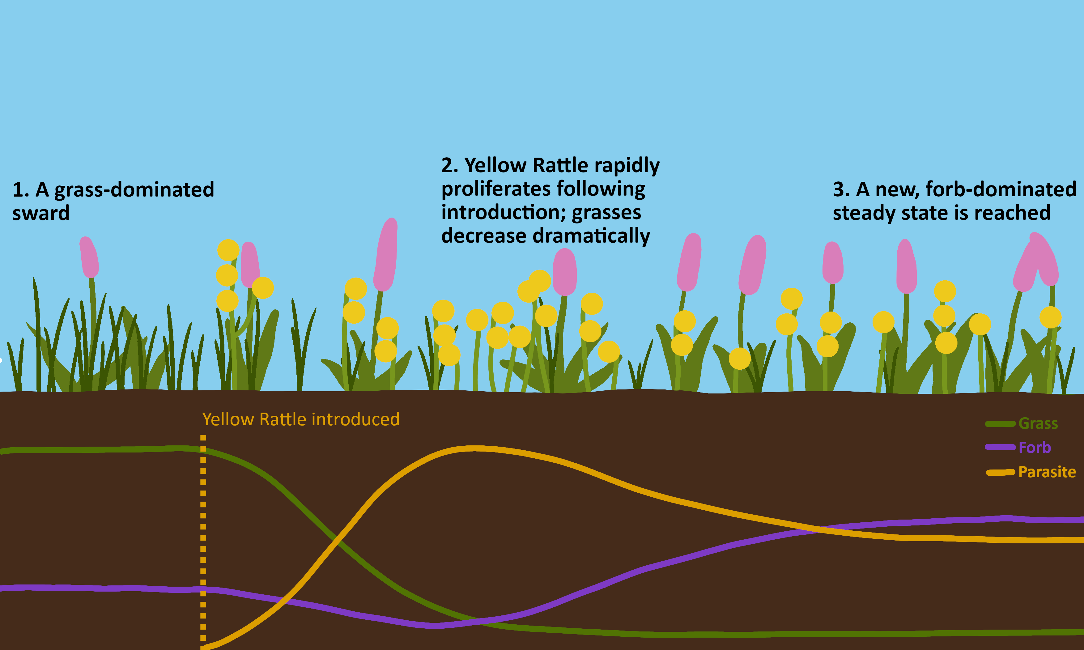
On the other hand, the dynamics do provide a nice illustration of how hemiparasites can affect plant communities. I used this to create an illustration of the ideal case of Yellow Rattle introduction:

References

1. D. D. Cameron, A. White, J. Antonovics, Parasite–grass–forb interactions and rock–paper– scissor dynamics: predicting the effects of the parasitic plant Rhinanthus minor on host plant communities. Journal of Ecology. 97, 1311–1319 (2009).
2. J. S. Petermann, A. J. F. Fergus, L. A. Turnbull, B. Schmid, Janzen-Connell Effects Are Widespread and Strong Enough to Maintain Diversity in Grasslands. Ecology. 89, 2399–2406 (2008).